[Paper Review] Kinetic Component Analysis
Ship Portrait - "Star Geiranger" by Louis Vest
Imagine you’re a spy who was assigned to track an arms shipment. You attach a tracking device to the cargo ship carrying the armaments just before it leaves the harbour. Your laptop starts blinking coordinates on its screen, but you soon notice a small problem - the coordinates appear on somewhat random spots. Something is interfering with the tracking signal, causing it to send distorted locations. Still, you can see that the location dots are generally trending towards the northwest. You think you know where the ship is headed.
Discerning the direction of such a cargo ship shares many similar challenges as deducing the direction of financial asset prices. The ship’s location is analogous to each asset’s fair value, which we define as the equilibrium price that attracts the same number of buyers and sellers. As with the ship’s location, we can’t directly observe fair value - prices printed on ticker tapes deviate randomly from fair value, owing to the random arrival times of buyers and sellers.
If fair value never changes, deducing it would merely require a little patience. We’d only need to collect a few weeks’ worth of price prints, and then calculate their average. What makes this problem challenging is that, as with discerning the cargo ship’s location, fair value changes constantly. When printed prices change, we therefore need to distinguish between fleeting changes caused by random arrival of buyers and sellers, and permanent changes stemming from movements in fair prices.
Many real world problems similarly involve having to locate and forecast moving targets using noisy observations. One elegant statistical model that solves such problems is the ‘Kalman Filter’. Invented around 1960, the model has been used, among other applications, by the Apollo program to help navigate rockets.
The unobservable numbers in Kalman filters, such as the true coordinates of the cargo ship or the fair value of a stock, are referred to as latent variables. A Kalman filter can contain multiple latent variables, not all of which need to influence observations directly. A ship’s velocity, for instance, can be a latent variable that doesn’t influence GPS coordinates directly, but does so indirectly by affecting the ship’s position. Upon receiving each new observation, Kalman filters shift the values of latent variables.
Just how far to shift the variables depends on the noisiness of the dataset. When data is noisy, new observations will pop up randomly inside a large area surrounding an anchor point. In such cases, Kalman filters would receive each new observation with skepticism, crediting most of the changes to fleeting observation errors, and shift latent variables only by small increments. Conversely, if the data is not very noisy, Kalman filters will shift variables more aggressively upon each new observation. The magic of statistics is used to determine the precise amount to shift, as well as to infer the values of the latent variables. Inferring latent variable values can be thought of as separating signals from noise.
Financial datasets are typically very noisy, making them prime candidates for Kalman filters to extract signals from. Those signals, such as the fair value estimates of stocks, would be useful for many applications. But finance papers that utilize Kalman filters are few and far between. One rare paper that does use Kalman filters is titled ‘Kinetic Component Analysis’ by Drs. Marcos Lopez de Prado and Riccardo Rebonato, wherein the authors present an augmented version of a popular form of Kalman filters.
The popular form contains two latent variables: position and velocity. The model assumes that velocity evolves randomly, free of influence from other variables. Position, on the other hand, is influenced by the current velocity, but also moves randomly besides. A ship’s position is not only determined by its speed and direction (i.e. velocity), but also by the erratic motions of waves. Observed data is modelled as an approximation centered around its position. Such data is not influenced directly by velocity.
De Prado and Rebonato’s model introduces the ‘acceleration’ latent variable in addition to the two existing variables. Acceleration evolves randomly over time, and influences both velocity and position. As with velocity, acceleration doesn’t influence observations directly. Neither velocity nor position influences acceleration. Though designed with financial applications in mind, the dynamics between acceleration, velocity and position are identical to those found in physics.
The introduction of acceleration improves Kalman filters’ capabilities for some datasets, but not for all. Some phenomena, such as a gambler’s winnings in a casino, don't feature any directional consistency, and including acceleration in such cases would only clutter models without providing any benefits. But for phenomena that show at least some directional consistency, the presence of acceleration can improve the effectiveness of the models significantly. The authors included a helpful summary data in Table 2 that shows which datasets exhibit acceleration.
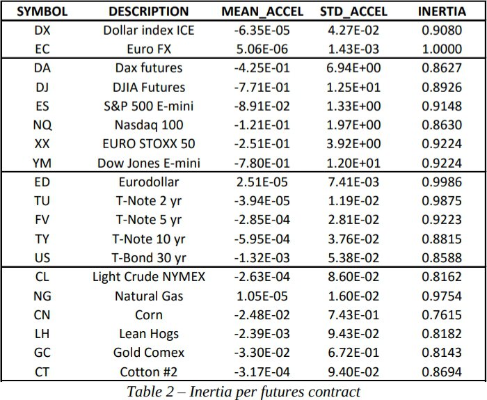
The ‘Inertia’ column shows the proportion of time when acceleration was insignificant (i.e. close to 0). The Euro FX and Eurodollar datasets never display any meaningful acceleration, and thus wouldn’t benefit from de Prado and Rebonato’s enhancements. Natural gas and T-Note 2 yr appear to exhibit acceleration on rare occasions, but we must question whether those instances were flukes. Given enough time, even gamblers will go on winning streaks, and appear to accelerate their winnings.
The remaining datasets, including the major equities indices, display acceleration often enough that its presence should improve the model’s effectiveness. There is one caveat, however. The analysis period runs from 2007 to 2012. Many machine learning techniques have seen their effectiveness drop since this period, as other market participants adopted similar techniques. The analysis period also includes the financial crisis, an atypical period during which time many machine learning techniques performed unusually well. I suspect acceleration has exerted a weaker influence since 2012.
We can improve Kalman filters further by building on the form suggested by de Prado and Rebonato. One way to achieve this is by incorporating other latent variables that evolve alongside position, velocity and acceleration. For instance, many people believe that equities tend to move in conjunction with money supply. One can express this view by creating a latent variable that represents money supply, and configuring it so it influences the latent variable that represents an equity indices’ fair value.
Another way to enhance Kalman filters is to introduce ‘control variables’. Whereas latent variables are “internal” to the model in which each step of their evolution is predicted by the model itself, control variables are “external” to the model. In other words their states are determined by outside forces without the model having the faintest clue about the process that generates those states. Though generated outside of the model, control variables can nonetheless exert influence on latent variables. An example of a control variable is the month of the year. The month doesn’t change according to a random process that evolves alongside with equities indices, so it shouldn’t be modeled as a latent variable. But many traders believe that specific months exert influence on stock prices (e.g. ‘Sell in May and go away’, ‘Santa Claus rally’), so it can be incorporated as a control variable.
I feel that de Prado and Rebonato underplayed the potential of control variables. They defined the variables as those within the modeler’s control, and cited the Federal Reserve’s capacity to change interest rates as an example variable that’s only available to the Federal Reserve. But control is actually irrelevant. You only need to be confident that an event will occur. If you’re willing to bet that the Federal Reserve will change interest rates in a certain direction, you can incorporate that information as a control variable.
De Prado and Rebonato compare their version of Kalman filter against two competing methods that extract signals from noise. The first method, called the Fast Fourier Transform (FFT) method, decomposes datasets into waves of different frequencies. FFTs are most effective when data exhibits a repeated pattern. Pop songs, for example, consist of verses and choruses that alternate in predictable order. Each verse and chorus span a consistent number of measures, and each measure is marked by the same sequence of beats. It therefore comes as no surprise that FFTs have been used by MP3 codecs to compress music into smaller files, by only keeping the most important signals and discarding the rest.
FFTs, however, are not effective when patterns don’t repeat themselves, or when they repeat irregularly. It’s therefore not clear whether FFTs are suitable for financial datasets. While some technical analysts argue that asset prices follow wavelike patterns, those waves have irregular shapes at best. Asset prices can also jump, and jumps can’t be approximated by a wave of any frequency. Kalman filters, which don’t struggle with such problems, have been found to outperform FFTs.
The other competitor of Kalman filters examined is the LOWNESS algorithm. This method fits linear regressions within a moving window of a dataset. Take, for example, a dataset that ranges from January to October. If we applied LOWNESS using moving windows that span 1 month, we’d first fit a linear regression using data from Jan 1 to Feb 1. We’d then slide the window to encompass data from Jan 2 to Feb 2, and fit another linear regression. We’d continue in like manner until we fit the last linear regression using data from Sep 30 to Oct 31.
LOWNESS appears to be able to extract similar signals as Kalman filters, but it suffers from a big flaw - it can’t generate forecasts. There is a way around this flaw - we could take the line fitted in the last window ( Sep 30 to Oct 31) and extend it into the future. But this method would have trouble predicting several steps ahead because its forecasts are based only on the last window and ignore insights gained from the vast majority of data that exist outside of that window. KCA doesn’t suffer from this problem, and would likely perform better than LOWNESS, particularly on multi step-ahead forecasts.
I don’t believe the authors intended to propose a form of Kalman filter that would be used without modification in the real world. Rather, I believe the authors wrote this paper to highlight the amazing potential of Kalman filters, to prompt practitioners to devise custom Kalman filters with problem-specific modifications, and to encourage more academics to utilize it when writing finance papers. I hope the authors will succeed.


